
Most churn models answer a simple question: “Will this customer leave?” But business teams often need a better one: “When are they likely to leave?” Time-to-event thinking changes the way churn is measured and managed. Instead of producing a single churn probability, survival analysis estimates how churn risk evolves over time and how long customers typically remain active. This is especially useful for subscription businesses, telecom, lending, insurance, SaaS, marketplaces, and any product where customers may churn at different points in their lifecycle.
Survival curves let you quantify retention in a way that is easy to explain: the curve shows the probability that a customer is still active after a certain number of days or months. When you connect this to product usage, support experience, pricing changes, and customer profiles, you can predict churn timing, prioritise interventions, and measure whether retention actions actually shift outcomes. Professionals exploring data analytics courses in Hyderabad often use churn as a capstone topic because it combines statistics, product reasoning, and business impact.
Understanding Time-to-Event Data and Censoring
In churn prediction with survival analysis, the “event” is churn (cancellation, inactivity beyond a threshold, contract termination, or account closure). The “time” is the duration from a start point (signup, first purchase, activation, or last renewal) until churn occurs.
A crucial difference from standard classification is censoring. Many customers have not churned by the end of your observation window. You do not want to label them as “non-churn” forever; you only know they survived up to a certain date. Survival analysis handles this naturally by treating them as right-censored observations. This preserves information and avoids bias that happens when you force a binary label too early.
Key elements you define upfront:
- Time origin: onboarding date, first payment date, or activation date
- Event definition: explicit cancellation, or “inactive for 60 days”
- Observation window: the last date included in modelling
- Censoring rule: customers still active on the last date are censored
These choices shape your survival curve and must reflect operational reality.
Survival Curves and the Kaplan–Meier Estimator
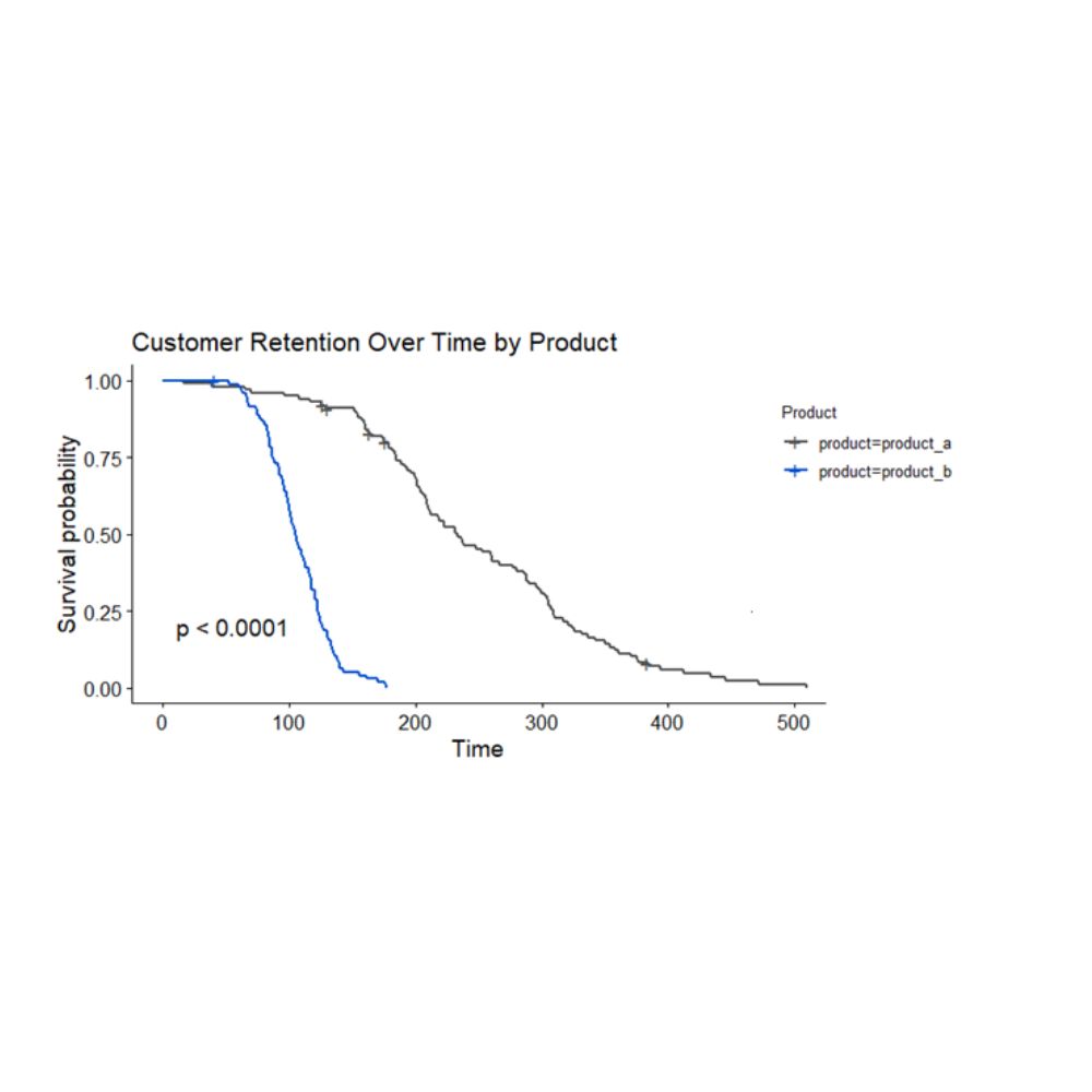
A survival curve answers: “What proportion of customers remain active beyond time t?” The Kaplan–Meier (KM) estimator is the starting point. It estimates the survival function as a stepwise curve that drops when churn events occur.
What you can learn from KM curves:
- Early-life churn: steep drops in the first weeks may signal onboarding friction
- Mid-life churn: drops after trial-to-paid transitions or renewals may signal pricing/value mismatch
- Segment differences: separate curves for cohorts (channel, plan, region, acquisition campaign) show which groups retain better
For example, if customers acquired via discounts show a faster decline after month 2 than customers acquired via referrals, you may redesign incentives or onboarding for that cohort. This kind of cohort storytelling is commonly practised in data analytics courses in Hyderabad because it links statistical outputs to actionable decisions.
Moving from Descriptive Curves to Predictive Churn Risk
Kaplan–Meier curves are descriptive. To predict churn timing for individuals and quantify drivers, you typically use a regression-style survival model.
Cox Proportional Hazards model (Cox PH)
Cox PH estimates how features change the hazard rate (instantaneous churn risk). It does not require specifying the baseline hazard shape, which makes it flexible. Outputs are often expressed as hazard ratios. A hazard ratio above 1 means higher churn risk; below 1 means lower churn risk.
Common feature groups:
- Engagement: sessions per week, feature adoption, recency of usage
- Service experience: ticket volume, resolution time, NPS/CSAT signals
- Commercial: plan type, discounts, tenure, payment failures
- Customer profile: industry, business size, geography, device type
If the proportional hazards assumption is violated (the effect changes over time), you can use time-varying covariates or alternative models.
Accelerated Failure Time (AFT) models
AFT models directly estimate how factors speed up or slow down time-to-churn. They can be easier to interpret for some stakeholders because they relate to expected survival time rather than hazard.
Whichever approach you choose, survival models let you produce:
- A personalised survival curve per customer
- The probability of churn within the next k days
- Rankings for retention outreach based on time-sensitive risk
Evaluation, Monitoring, and Practical Deployment
Survival modelling requires evaluation metrics suited to time-to-event data. Common ones include:
- Concordance index (C-index): measures ranking quality of predicted risks
- Time-dependent AUC: evaluates discrimination at specific horizons
- Calibration over time: checks whether predicted survival matches observed survival
Deployment considerations that prevent common mistakes:
- Data leakage control: do not use features that occur after the churn event date
- Stable time origin: keep consistent definitions across cohorts
- Refresh cadence: churn dynamics change after pricing updates, seasonality, or product releases
- Actionability: translate predictions into playbooks (onboarding nudges, success calls, billing fixes)
Teams building a portfolio from data analytics courses in Hyderabad often demonstrate value by showing how an intervention shifts survival curves for a treated group versus a control cohort, rather than only reporting a single churn percentage.
Conclusion
Survival curves turn churn prediction into a time-aware, decision-friendly discipline. By modelling retention as a probability over time, you can handle censored customers correctly, compare cohorts with Kaplan–Meier curves, and identify churn drivers using Cox or AFT models. The result is more than a churn score: it is a practical view of when customers are at risk and what levers can extend their lifetime. When implemented with careful definitions, clean feature timing, and time-based evaluation, survival analysis becomes one of the most reliable ways to forecast attrition and guide retention strategy.